To begin, start Explorer CE and select New Project:
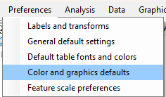
We first need to specify the default heat map colors that are going to be used. Thus, in the Preferences pull-down menu, select Color and graphics defaults:
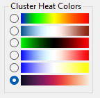
Next, on the left side of the panel that appears, select the radiobutton at the bottom of the Cluster Heat Colors options:
Then click on the Apply button:
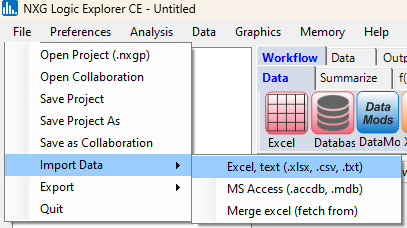
Select Import Data, then Excel:
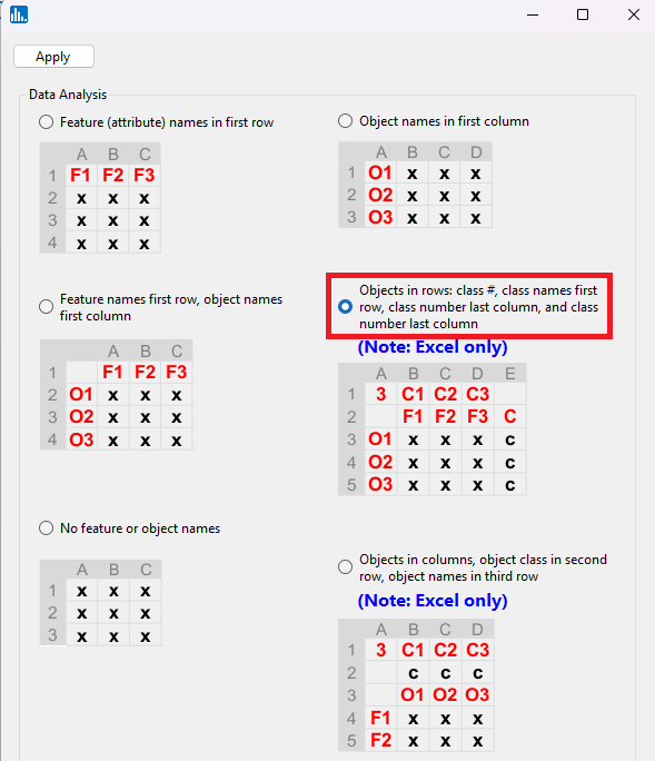
Select the radiobutton for opening an Excel file that contains a class feature, which also has the number of classes and class names in the first row of the spreadheet:
This tutorial uses expression values for p=23 mRNAs which are strongly predictive of n=63 SRBCTs in 4 diagnostic classes (Ewing's sarcoma, neuroblastoma, Burkitt's lymphoma, and rhabdomyosarcoma).
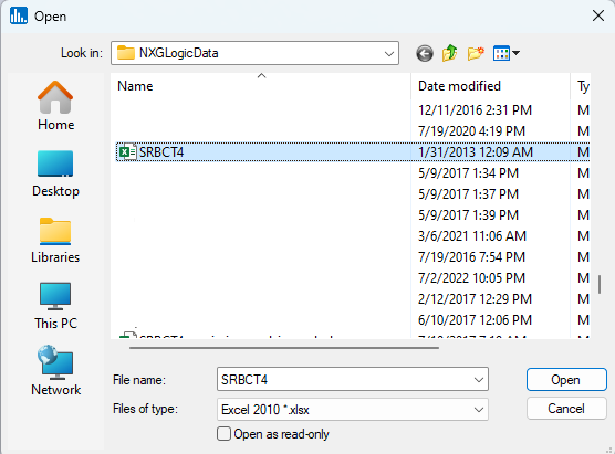
In the file-open dialog window, locate the SRBCT4.xlsx file that is distributed with Explorer CE and double-click on it:
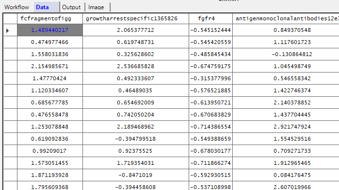
You will then see that the data are loaded in the datagrid:
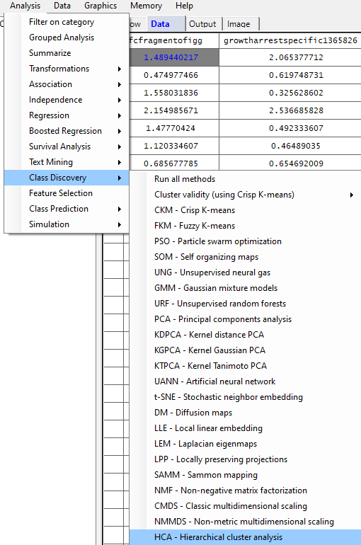
Next, in the Analysis pull-down menu, select Class Discovery, then HCA - Hierarchical cluster analysis:
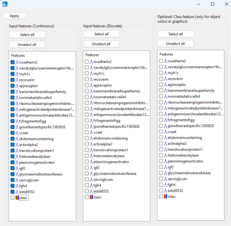
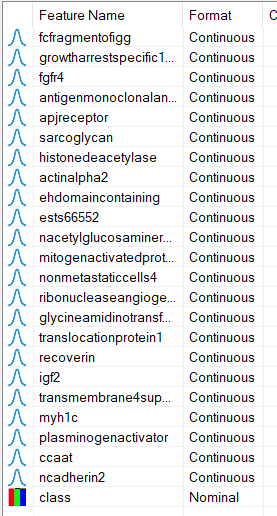
In the next popup window, select all of the features except the class feature:
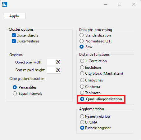
In the parameter popup window, select Quasi-diagonalization, and then click on Apply:
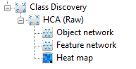
After the run has completed, you will notice the following icons in the treeview to the left. Click on the Heat map icon:
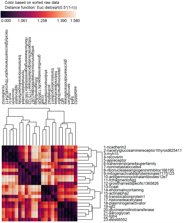
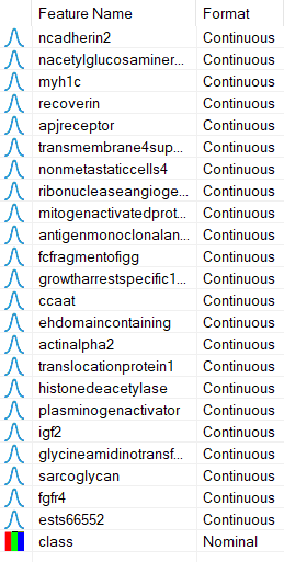
The heat map is shown below. Notice that the feature-by-feature matrix is now diagonally dominant and symmetric. However, this is not a correlation matrix, it is a matrix based on Euclidean distance of sqrt(0.5*1-r)). We generate a correlation matrix next - see below.
In addition, the order of the features in memory were re-arranged according to the order shown in the cluster heat map.
Since the order of the input features is now changed, we can straightforwardly run a correlation analysis and generate a correlation matrix as well as a "significance heat map" to reveal that the greatest correlation coefficients are near the diagonal of the correlation matrix.
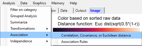
From the Analysis pull-down menu, select Association, then Correlation, Covariance, or Euclidean distance:
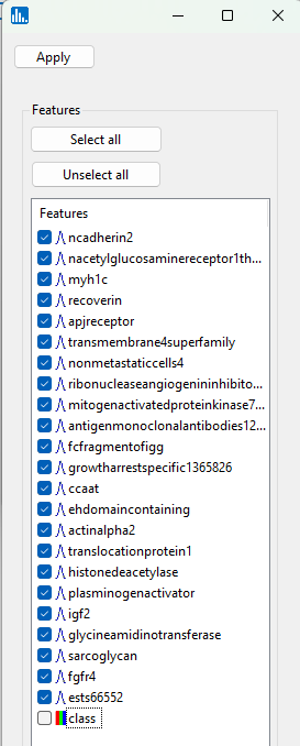
Select all the re-ordered features, except the class feature, and then click on Apply:
After the correlation run, the following icons will be visible:
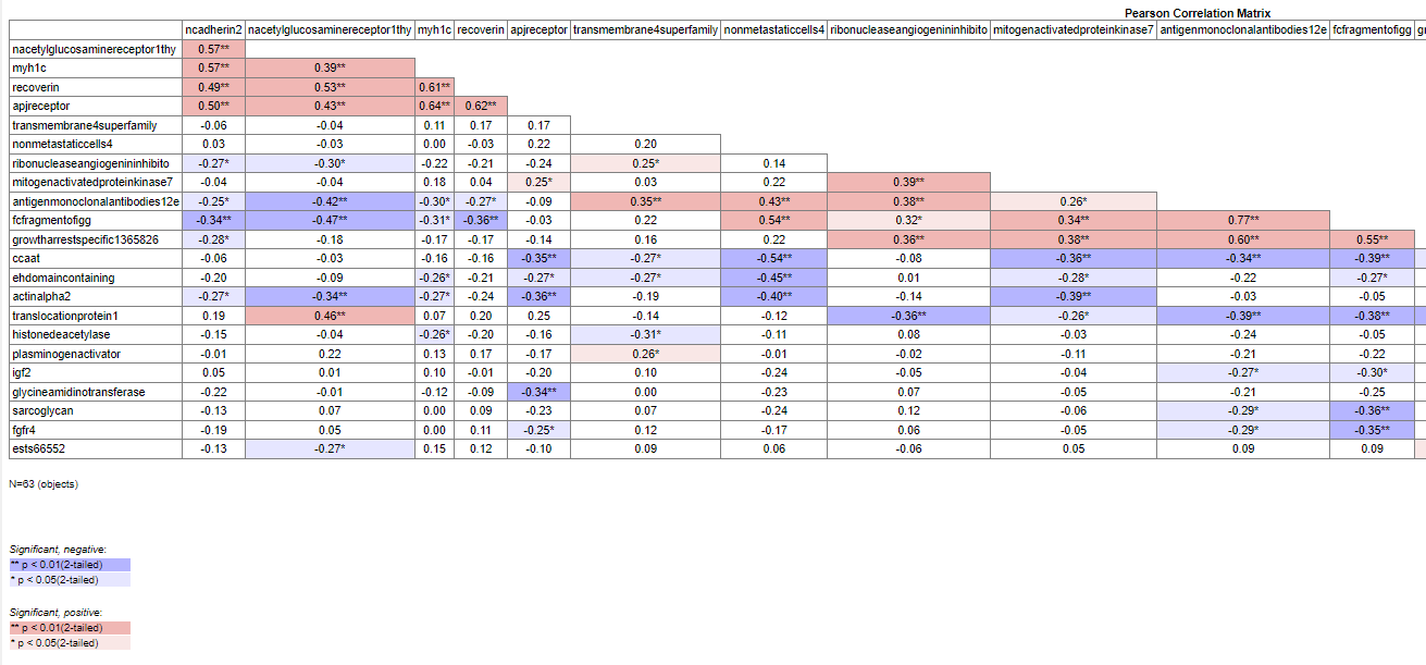
Click on the Pearson correlation (html) icon, which will show the html version of the correlation matrix. Notice that a majority of the greatest and most significantly positive (r>0) coefficients are near the diagonal of the correlation matrix. (to zoom out from the html table, select Cntl and use your mouse-wheel).
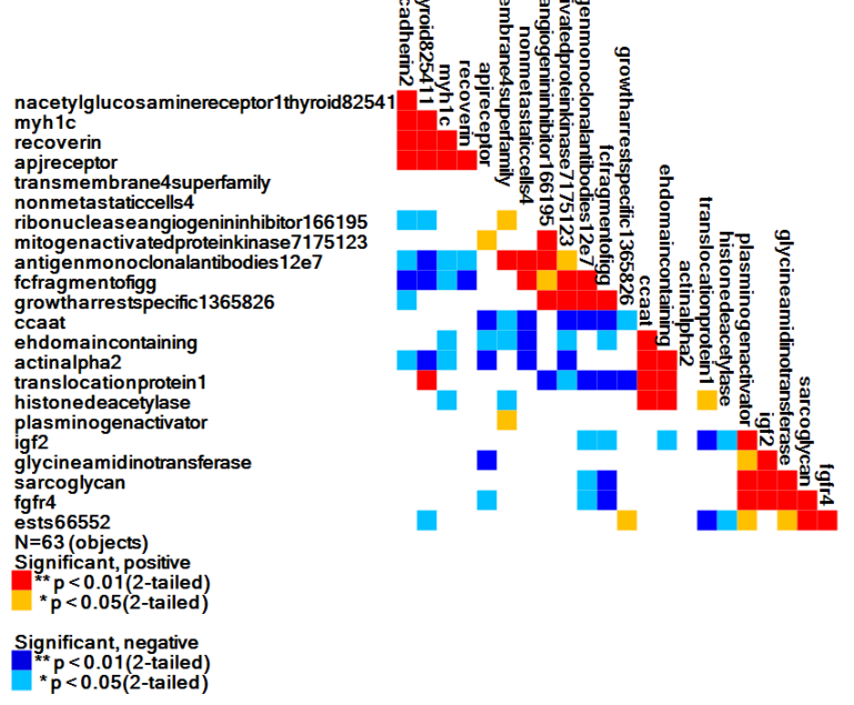
Next, click on the Pearson correlation icon (the 2nd icon) and you will see a heat map showing the correlation matrix with color-coding related to significance test results for each coefficient. Red-colored coefficient cells in the image represent positive correlation coefficients whose p-values are significant at the 0.01 level. This image is perhaps the best one to use to show a diagonally dominant correlation matrix based on quasi-diagonalization, since the original cluster heat map (shown above after hierarchical cluster analysis - HCA) is based on Euclidean distance.