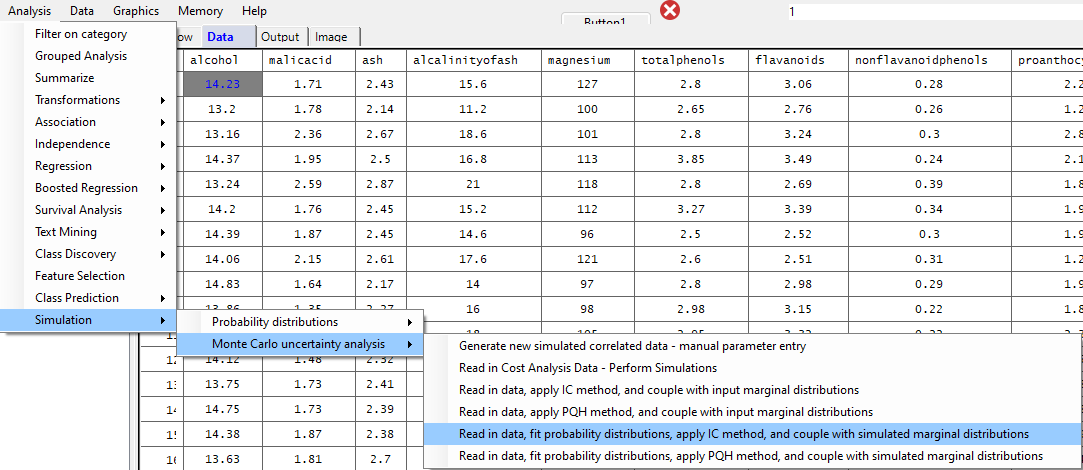
By pull-down menu:
This example run involves first reading in the wine.xlsx dataset, fitting the probability distributions of all the continuously-scaled input features, assessing the correlation structure, and implementing the Iman & Conover method for quantile generation of correlated non-normally distributed features. First, open the wine.xlsx dataset. Next, in the Analysis pull-down menu, select Monte Carlo uncertainty analysis, then Read in data, fit probability distributions, apply IC method, and couple with simulated marginal distributions, as shown below:
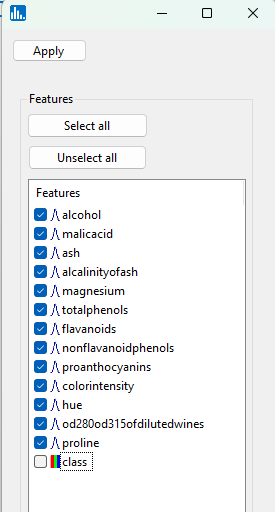
You will then see the following popup window for feature selection. Select all the continuous features as shown. Then click on Apply:
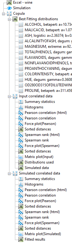
Once you click on Apply, the processing will commence and when done, the following icons will appear in the treeview:
The images below show the result for clicking on the various output icons:
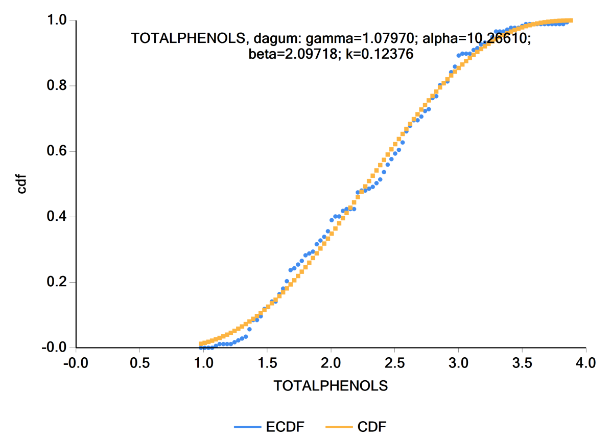
Below is a plot of the empirical cumulative distribution (ecdf) and the fitted cdf for totalphenols. As you can note, the 4-parameter Dagum distribution was the best fitting distribution. The parameters for the Dagum distribution are listed.
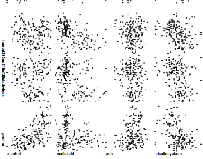
Below is the matrix plot for the input data:
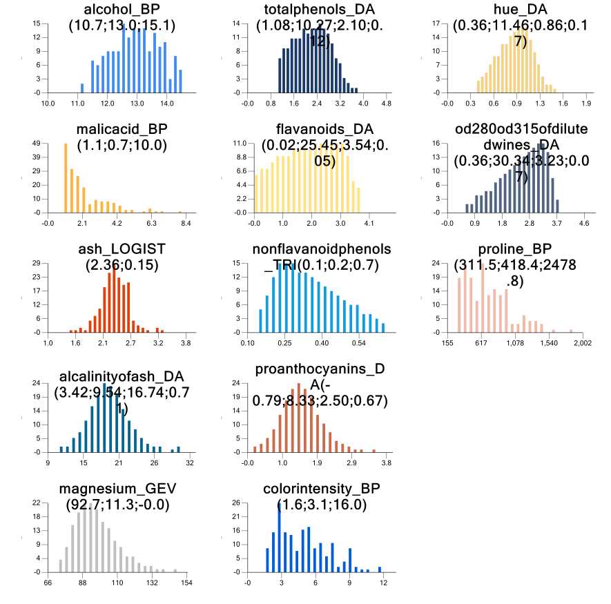
The histograms of the fitted-correlated data are shown. This plot is available when clicking on the "Histogram" icon in the bottom group of icons under "Correlated" data.
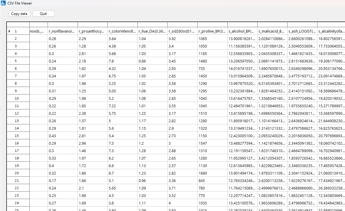
If you click on the "Fitted results" icon at the very bottom of the icon list, you will see the raw data that were read in on the left side of the datagrid (feature names are preceded by "r_", indicating read in), and on the right side of the datagrid are the simulated correlated data based on the best fitting probability distributions, where feature names are preceded by "s_" to denote simulated. The simulated feature values also take on the correlation structure of the input features.