


There are many ways in which an artificial neural network (ANN) can break down and not perform well. In this blog, we go through some of the essential requirements for getting a feed-forward ANN to work properly for a typical classification problem. The dataset chosen was the "Large Soybean Database" dataset from the UCI Machine Learning repository. (ref: R.S. Michalski and R.L. Chilausky. "Learning by Being Told and Learning from Examples: An Experimental Comparison of the Two Methods of Knowledge Acquisition in the Context of Developing An Expert System for Soybean Disease Diagnosis." Int. J. of Policy Analysis and Information Systems. 4(2); 1980.)
There are 15 classes and 35 categorical attributes in this dataset, some nominal and some ordered. We make the assumption that the data can be directly input into an ANN without creating k-1 dummy indicators (0,1) for each level of the factors, which would result in more than 100 binary features. (this could be done, but was not for the sake of efficiency). The number of objects was n=266 (there were n=307 original objects but we dropped records with missing data).
The 15 classes are:
diaporthe-stem-canker, charcoal-rot, rhizoctonia-root-rot, phytophthora-rot, brown-stem-rot, powdery-mildew, downy-mildew, brown-spot, b acterial-blight, bacterial-pustule, purple-seed-stain, anthracnose, phyllosticta-leaf-spot, alternarialeaf-spot, frog-eye-leaf-spot.
The 35 features are:
1. date: april,may,june,july,august,september,october.
2. plant-stand: normal,lt-normal.
3. precip: lt-norm,norm,gt-norm.
4. temp: lt-norm,norm,gt-norm.
5. hail: yes,no.
6. crop-hist: diff-lst-year,same-lst-yr,same-lst-two-yrs,same-lst-sev-yrs.
7. area-damaged: scattered,low-areas,upper-areas,whole-field.
8. severity: minor,pot-severe,severe.
9. seed-tmt: none,fungicide,other.
10. germination: 90-100%,80-89%,lt-80%.
11. plant-growth: norm,abnorm.
12. leaves: norm,abnorm.
13. leafspots-halo: absent,yellow-halos,no-yellow-halos.
14. leafspots-marg: w-s-marg,no-w-s-marg,dna.
15. leafspot-size: lt-1/8,gt-1/8,dna.
16. leaf-shread: absent,present.
17. leaf-malf: absent,present.
18. leaf-mild: absent,upper-surf,lower-surf.
19. stem: norm,abnorm.
20. lodging: yes,no.
21. stem-cankers: absent,below-soil,above-soil,above-sec-nde.
22. canker-lesion: dna,brown,dk-brown-blk,tan.
23. fruiting-bodies: absent,present.
24. external decay: absent,firm-and-dry,watery.
25. mycelium: absent,present.
26. int-discolor: none,brown,black.
27. sclerotia: absent,present.
28. fruit-pods: norm,diseased,few-present,dna.
29. fruit spots: absent,colored,brown-w/blk-specks,distort,dna.
30. seed: norm,abnorm.
31. mold-growth: absent,present.
32. seed-discolor: absent,present.
33. seed-size: norm,lt-norm.
34. shriveling: absent,present.
35. roots: norm,rotted,galls-cysts.
The class priors (counts) are:
1. diaporthe-stem-canker: 10
2. charcoal-rot: 10
3. rhizoctonia-root-rot: 10
4. phytophthora-rot: 40
5. brown-stem-rot: 20
6. powdery-mildew: 10
7. downy-mildew: 10
8. brown-spot: 40
9. bacterial-blight: 10
10. bacterial-pustule: 10
11. purple-seed-stain: 10
12. anthracnose: 20
13. phyllosticta-leaf-spot: 10
14. alternarialeaf-spot: 40
15. frog-eye-leaf-spot: 40
Network architecture: To begin, the feed-forward, back-propagation based, single hidden-layer network structure included 35 input nodes, 23 hidden nodes, and 15 output nodes (Peterson et al., 2005). The trapezoidal pyramid rule was used for determining the number of hidden nodes in the hidden layer. The tanh activation function was used at the hidden nodes, and the logistic function was used for the output nodes. Normally, we would use the softmax function on the output-side, however, the predicted target values in the range [0,1] from the logistic function worked well for this dataset. MSE was used as the objective function. In summary, the straightforward architecture resulted in a 35-23-15 ANN.
Cross-validation: 10-fold cross validation was used in which objects were first shuffled (randomly permuted) when assigned into the 10 folds. This has to be done to prevent an ANN from learning based on the order of training objects. During training, objects in folds 2-10 were used for training, while objects in the first fold were used for testing. For each test fold, we swept through the training objects 200 times (epochs), and updated connection weights for each object ("online" training). This was repeated for each of the remaining test folds. Normally, we always rerun the entire 10-fold CV procedure a total of ten times, by shuffling objects before assigning them to the 10 folds, and then training and testing again -- resulting in what is called "ten 10-fold CV." We didn't pad the confusion matrix to determine predictive accuracy for this run, or calculate sensitivity, specificity, ROC-AUC, etc., since we only show how the changes made result in fluctuations in training and testing error.
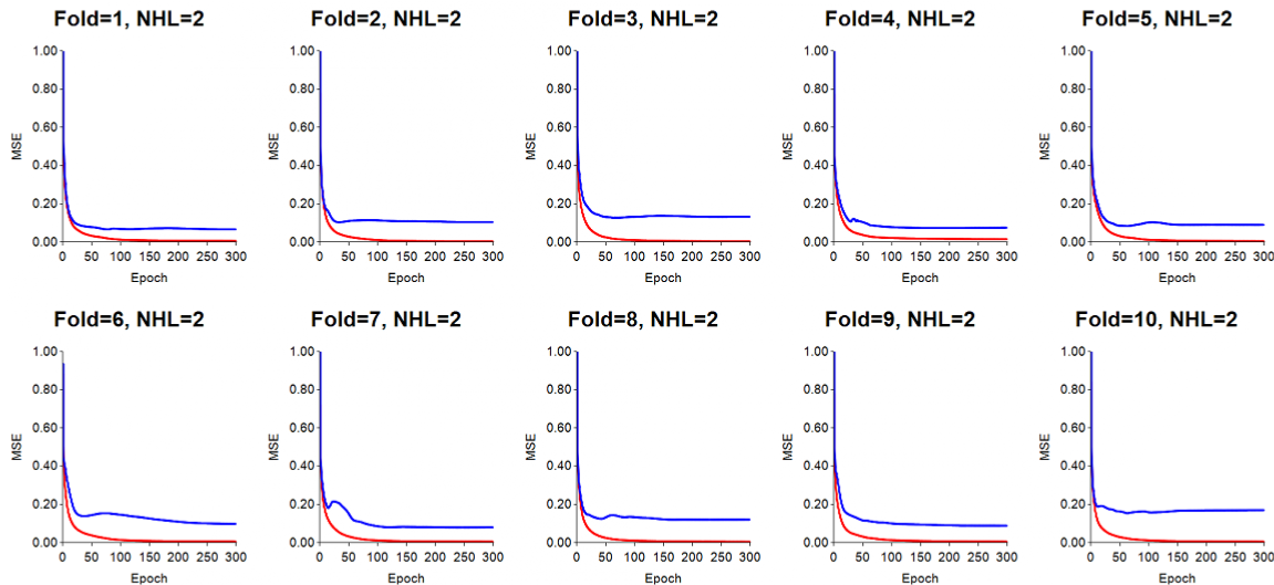
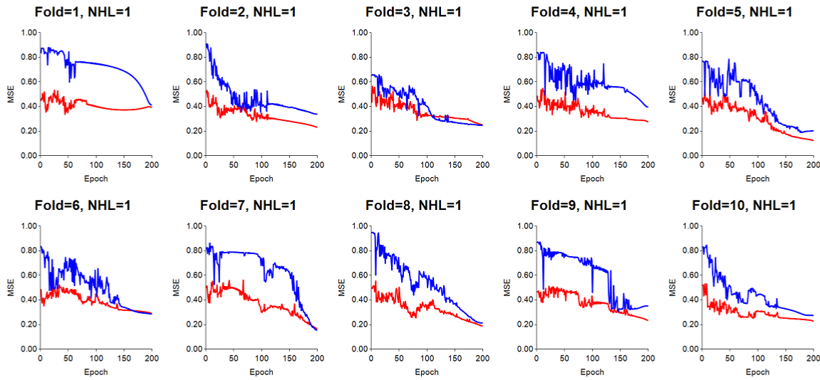
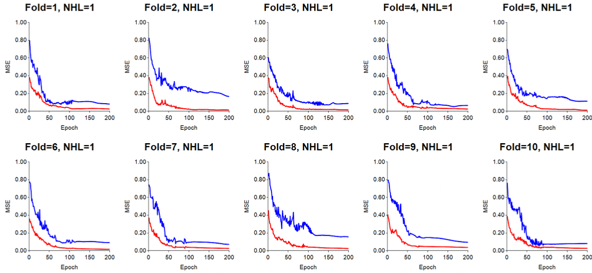
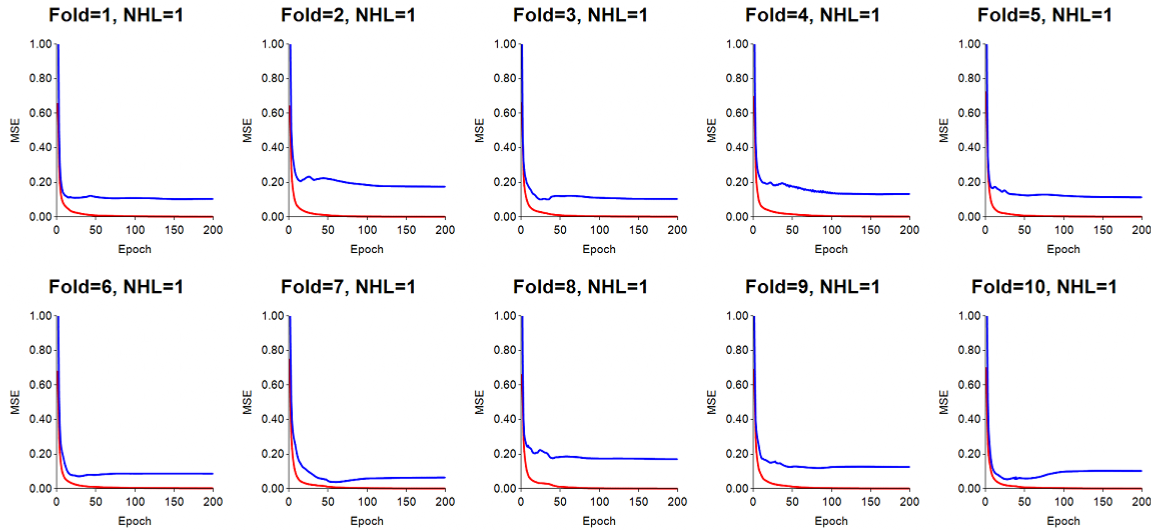
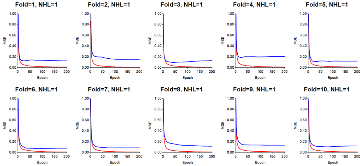
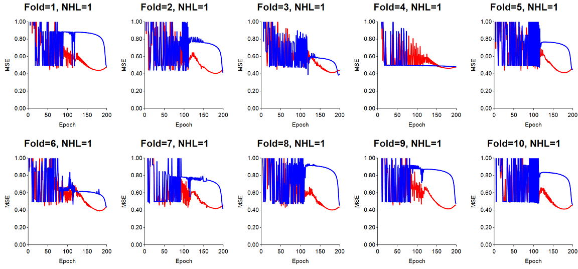
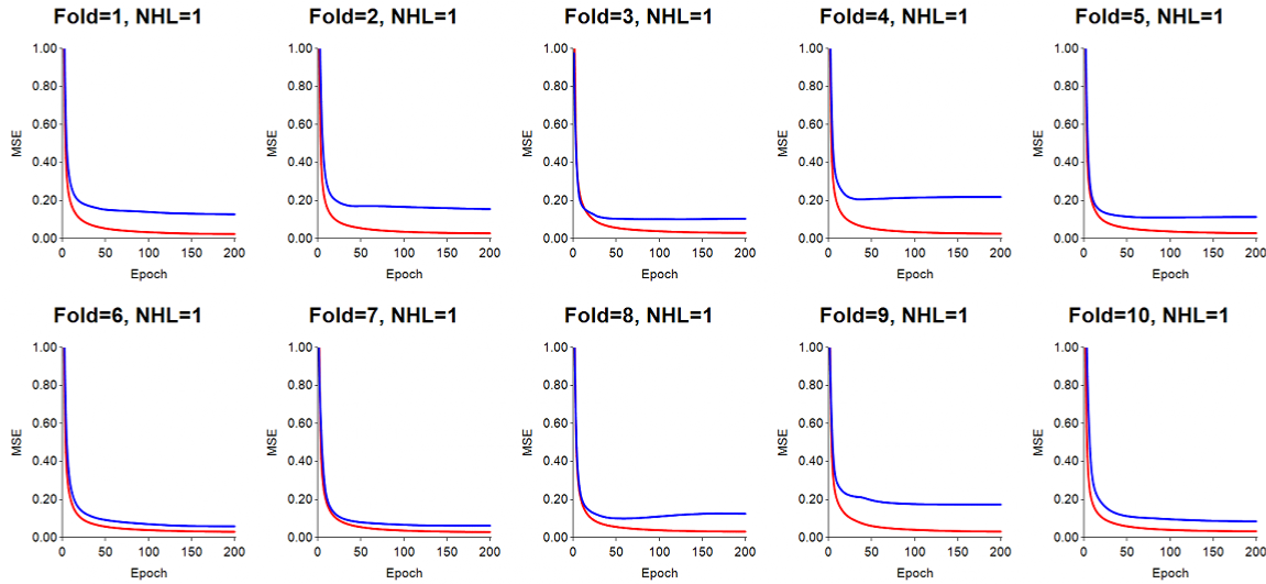
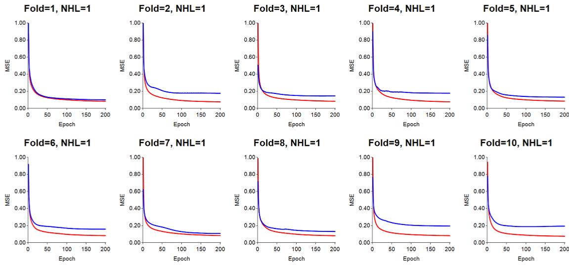
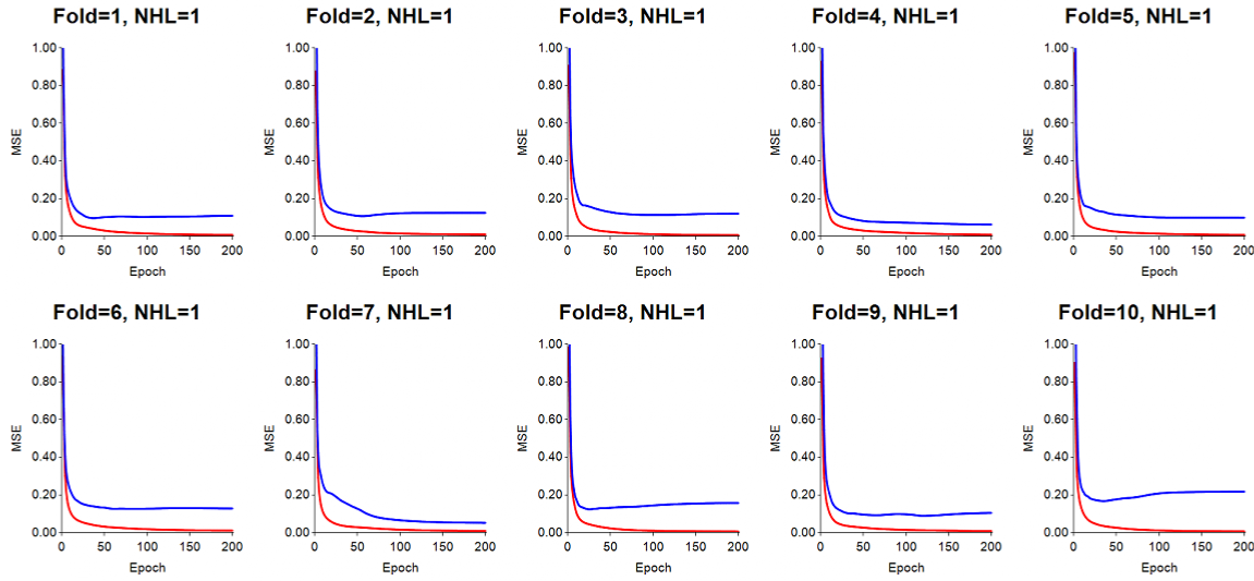
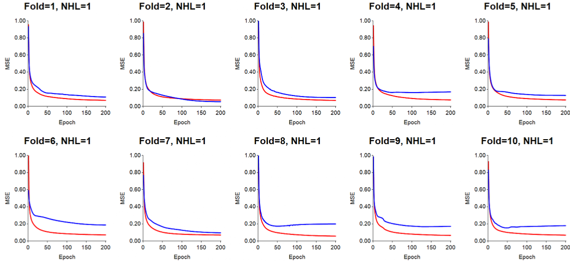
The following paragraphs and plots start with a poorly trained ANN, and gradually add changes to the parameters and training options to show what needs to be considered when training/testing with an ANN for classification analysis. In the plot titles, "NHL=" applies to the number of hidden layers used, and "Fold=" applies to the test fold being used. The red lines denotes the training error (MSE), while the blue lines represent the test error for objects left out of training.
Avoiding information leakage: When mean-zero standardization of features is introduced during the runs, it is important to note that the means and standard deviations obtained from training objects were used for standardizing the feature values of the test objects. Mean-zero standardization should never be run for a feature using the entire dataset, because information from test objects would then be commingled with information used in training. Thus, no statistics from test features are ever used for feature transformation of test objects.
Learning rate much too high (LR=0.6): for this run, LR was set to 0.6, which proved to make the gradient steps too large. The result is a training error (red) and test error (blue) which are very jumpy. Momentum was set to 0.7.
Learning rate still too high (LR=0.2): Even when the LR was 0.2, it was still too high, resulting in jumpy transitions of the error lines. Momentum was set to 0.7.
Learning rate acceptable (LR=0.05): When the LR=0.05, an ANN has a better chance of learning the training data more smoothly. However, we have learned that the larger the problem, i.e., the greater the number of objects used for training and testing, the lower LR should be. Thus 0.02 or even 0.01 have shown reliable results. We have also seen cases where the test error decreases with the learning rate, such that the test error, for example, was lower when LR=0.02 when compared with test error when LR=0.05. For this run, momentum was set to 0.7.
Mean-zero standardization of input features: With the LR set to 0.05, in this run we performed mean-zero standardization of all of the input features. The results obtained indicate quite smooth values of training and test error over the data sweeps (epochs). Momentum was set to 0.7.
Mean-zero standardization with lower LR=0.02: By reducing the LR to 0.02, some of the folds displayed lower test error. In addition, some slight jumpyness is also removed as training and testing proceed through the epochs. Momentum was set to 0.7.
Lowering momentum can reduce test error: In the run results shown above, we used a momentum value of 0.7. Using the same LR, we next lowered the momentum to 0.1, and the results indicate that for some test folds, the test error actually decreased. How an ANN responds to parameter settings, and which parameter settings are optimal for the given dataset can best be identified by using a grid search, which is what NXG Logic Explorer employs during ANN runs.
Running principal components analysis (PCA) on large feature sets can speed up learning and improve performance: In this run, PCA was run on the 35 features to extract 11 reduced dimensions (PCs) whose eigenvalues were greater than 1. The ANN's architecture was now 11-13-15. The 11 orthogonal PCs were then clamped to the input nodes of the ANN for training. The results obtained for a given dataset will depend on the amount of multicollinearity between the original input features. The soybean dataset has 35 features, and reduction of the dimensions resulted in use of 11 PCs for input, which did not change the results drastically. However, for very large datasets, use of PCA can be a tremendous cost savings in time complexity required for training, mostly because of the substantial reduction of connection weights which must be updated during back-propagation (Peterson and Coleman, 2005). For this run, LR=0.02, momentum=0.7.
Using K-means cluster analysis on objects can improve results: Next, we implemented K-means cluster analysis (K=5) with the original 35 features to extract 5 centers from objects in the training folds, each of which consisted of 35 means (averages) representing the average feature values of objects assigned to the 5 clusters during K-means training (see Peterson and Coleman, 2005) . For each test fold, we determined the object-to-center distance based on training centers, and used these distances as an additional set of 5 feature values for testing. This increased the total ANN input features to 40 (35+5), resulting in a 40-24-15 ANN architecture.
We have observed for large datasets that when training an ANN using CV, it is highly likely that objects in test folds could be quite different (randomly) from objects in the training folds, so we have found that by using the object-to-center distances during training and testing, we can adjust disparities among objects based on these distances. The object-to-center distances essentially inform the ANN that a given test object is closer or further away from objects used in training folds. This is the underlying principal of radial basis functions (RBFs), and how kernel regression classifiers work. For this run, LR=0.02, momentum=0.7.
Combining PCA and K-means cluster analysis improves performance further. At this point, we now use PCA to first reduce the original 35 features down to 11 orthogonal PCs, and then run K-means cluster analysis on the objects using the 11 PCs to obtain the K=5 centers (for the objects), and add the 5 K-means feature values for object-to-center distance to the 11 PCS to get 16 features. The network architecture is now a 16-15-15 ANN.
For very large datasets, when there several thousand objects in each test fold, we actually turn this approach on its head and run PCA and ANN training/testing CV for each K-mean cluster of objects. This helps enforce similar objects to be used in training and testing.
Fundamentally, for almost any dataset, there will usually be some kind of cluster structure in it; it may not be a rich cluster structure, but likely will be one that nevertheless reveals a moderate cluster structure. We also use a variety of cluster validity runs (with a lot of tricks) to determine the optimal value of K. For this run, LR=0.02, momentum=0.7.
Adding another hidden layer (i.e., NHL=2) does not help much: K-means cluster analysis (K=5) was employed on the original 35 features, and another hidden layer was employed using the tanh activation function. This resulted in a 40-29-21-15 ANN. Results indicate a slight reduction in overfitting, but not a substantial decrease in test error. This follows the general rule that additional hidden layers, in the main, do not help the performance of a typical feed-forward, back-propagation ANN.
Recall, there is a problem known as "vanishing gradients" which becomes more important as more hidden layers are used (see our blog on this). Essentially, beyond a certain number of hidden layers, depending on the number of features used and peculiarities of the dataset, the gradients involved with connection weights proximal to the input objects that are clamped to the ANN become too distant, i.e., disconnected, from the output nodes. This causes a "communication breakdown" between nodes in the ANN, and results in a breakdown in learning.